Text analysis of the 10th Republican Presidential candidate debate using R and the quanteda package
On 25 February 2016, the tenth debate among the Republican candidates for the 2016 Presidential election took place in Houston, Texas, moderated by CNN. In this demonstration of the quanteda package, I will show how to download, import, clean, parse by speaker, and analyze the debate by speaker.
The first step involves loading the debate into R. I got the debate from the New York Times publication of the transcript. It’s possible to copy and paste the text into a text editor, but because of headers, sidebar ads, and image captions, this necessitates a lot of cleaning afteward. To get around this, I printed the article to a pdf file, saved as republican_debate_2016-02-25.pdf.
To read this text, I then called the utility pdftotext, described in this post.
# convert the pdf into a character vector using pdftotext
transcriptText <- system2("pdftotext",
    args = "-layout ~/Desktop/republican_debate_2016-02-25.pdf -", stdout = TRUE)
The first command performs the conversion using the system2() call, sends this to “stdout”, which is assigned in R to transcriptText, a character vector consisting of one element per line of the text. The -layout argument to pdftotext preserves the formatting as printed in the original text. If we inspect the first 17 lines, we see the text, which includes tags for each speaker’s name in capitals, and parenthetical remarks such as “(APPLAUSE)” denoting non-text events.
# view the first 17 lines
cat(paste(transcriptText[1:17], collapse = "\n"))
##                       http://nyti.ms/1QJs7R9
##
##
##     ELECTION 2016    Nevada Results   Primary Calendar   Campaign Money
##
##
##
##
## Transcript of the Republican
## Presidential Debate in Houston
## FEB. 25, 2016
##
## Following is a transcript of the Republican debate, as transcribed by the
## Federal News Service.
##
##      BLITZER: We're live here at the University of Houston for the 10th
## Republican presidential debate. (APPLAUSE))
To make this a single text object, we will paste the lines together, joining them with the \n characters that separated them originally.
# paste together into one file
transcriptText <- paste(transcriptText, collapse = "\n")
To get only the text spoken by each candidate, we still need to remove some of the extra text at the beginning and the end of the article, and we need to remove the non-text markers for events such as applause. We can do this using a substitution of the text we wish to remove for the null string "", using gsub().
## clean up the text
# remove header
transcriptText <- gsub("^.+Federal News Service\\.\\s*", "", transcriptText)
# remove non-text transcript notes (list created by inspecting the text)
transcriptText <- gsub("\\s*\\((APPLAUSE|BELL RINGS|BELL RINGING|THE STAR-SPANGLED BANNER|COMMERCIAL BREAK|CROSSTALK|inaudible|LAUGHTER|CHEERING)\\)\\s*",
                       "", transcriptText)
# remove footer
transcriptText <- gsub("\\s+Find out.+2016 The New York Times Company\\s*$", "", transcriptText)
# inspect the the text
cat(paste(substring(transcriptText, 1, 1000), substring(transcriptText, 5000, 5655), collapse = "\n"))
## BLITZER: We're live here at the University of Houston for the 10th
## Republican presidential debate.BLITZER: An enthusiastic crowd is on hand here in the beautiful opera
## house at the Moore School of Music. Texas is the biggest prize next Tuesday,
## Super Tuesday, when 11 states vote, a day that will go a long way towards
## deciding who wins the Republican nomination.
##
##      We want to welcome our viewers in the United States and around the world.
## I'm Wolf Blitzer. This debate is airing on CNN, CNN International, and CNN in
## Espanol. It's also being seen on Telemundo and heard on the Salem Radio
## Network. Telemundo and Salem are our partners in this debate, along with the
## Republican National Committee.
##
##      We'd also like to welcome a very special guest with us here tonight. Ladies
## and gentlemen, the 41st president of the United States, George Herbert Walker
## Bush and former first lady Barbara Bush.Everyone here is looking forward to a lively debate. I'll be your moderator
## tonight. Joining me in ator Cruz?
##
##     CRUZ: Welcome to Texas.Here, Texas provided my family with hope. Here, my mom became the first
## in her family ever to go to college. Here, my dad fled Cuba and washed dishes,
## making 50 cents an hour to pay his way through the University of Texas. I
## graduated from high school at Second Baptist not too far away from here.
## CRUZ: When I ran for Senate, I promised 27 million Texans I would fight for
## you every day, and not for the Washington bosses.
##     And, I'll tell you, as I travel the state, Democrats tell me I didn't vote for
## you, but you're doing what you said you would do. And, as president, I will do
## the same.BLITZER: Mr. Trump.
Now that we have this as one “document”, we need to load it into the quanteda package for processing and analysis.
require(quanteda, warn.conflicts = FALSE, quietly = TRUE)
# make a corpus
transcriptCorpus <- corpus(transcriptText,
                           notes = "10th Republican candidate debate, Houston TX 2016-02-25",
                           source = "http://nyti.ms/1QJs7R9")
summary(transcriptCorpus)
## Corpus consisting of 1 document.
##
##   Text Types Tokens Sentences
##  text1  3114  30048      3306
##
## Source:  http://nyti.ms/1QJs7R9
## Created: Fri Feb 26 14:01:42 2016
## Notes:   10th Republican candidate debate, Houston TX 2016-02-25
Our goal in order to analyze this by speaker, is to redefine the corpus as a set of documents defined as a single speech acts, with a document variable identifying the speaker. We accomplish this through the segment() method:
## make into a corpus and segment by speaker
transcriptCorpus <- segment(transcriptCorpus, what = "tags", delimiter = "\\s*[[:upper:]]+:\\s+")
summary(transcriptCorpus, 10)
## Corpus consisting of 1 document.
##
##   Text Types Tokens Sentences
##  text1  3114  30048      3306
##
## Source:  http://nyti.ms/1QJs7R9
## Created: Fri Feb 26 14:01:42 2016
## Notes:   10th Republican candidate debate, Houston TX 2016-02-25
We can clean up the tags:
# tidy up whitespace from tags
docvars(transcriptCorpus, "tag") <- stringi::stri_trim_both(docvars(transcriptCorpus, "tag"))
# remove ":" from tag
docvars(transcriptCorpus, "tag") <- gsub(":", "", docvars(transcriptCorpus, "tag"))
# correct a misspelling of ARRASAS (NYT's fault!)
docvars(transcriptCorpus, "tag") <- gsub("ARRARAS", "ARRASAS", docvars(transcriptCorpus, "tag"))
# remove Cooper and "UNIDENTIFIED MALE
transcriptCorpus <- subset(transcriptCorpus, !(tag %in% c("MALE", "COOPER")))
# inspect the tags now
summary(transcriptCorpus, 10)
## Corpus consisting of 565 documents, showing 10 documents.
##
##     Text Types Tokens Sentences     tag
##   text11    14     15         2 BLITZER
##   text12   157    260        32 BLITZER
##   text13    16     17         2 BLITZER
##   text14    24     28         4 BLITZER
##   text15   116    200        24 BLITZER
##   text16    68     92        10  CARSON
##   text17     3      3         1 BLITZER
##   text18    98    164        19  KASICH
##   text19     3      3         1 BLITZER
##  text110    92    163        17   RUBIO
##
## Source:  http://nyti.ms/1QJs7R9
## Created: Fri Feb 26 14:01:42 2016
## Notes:   segment.corpus(segment.corpus)segment.corpus(transcriptCorpus)segment.corpus(tags)segment.corpus(\s*[[:upper:]]+:\s+)
# tabulate the speech acts by speaker
table(docvars(transcriptCorpus, "tag"))
##
## ARRASAS    BASH BLITZER  CARSON CELESTE    CRUZ  HEWITT  KASICH   RUBIO
##      24      26     108      15       1      75      26      26     100
##   TRUMP
##     164
Now we can start to perfom some analysis on the text. Who spoke the most in the debate, in words?
# who spoke the most?
par(mar = c(5, 6, .5, 1))
barplot(sort(ntoken(texts(transcriptCorpus, groups = "tag"), removePunct = TRUE)),
        horiz = TRUE, las = 1, xlab = "Total Words Spoken")
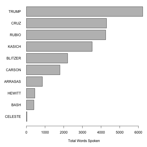
The ntoken() function does the work here of counting the tokens in the vector of texts returned by the call to transcriptCorpus, groups = "tag", which extracts the texts from our segmented corpus and concatenates all texts by speaker. This results in a vector of the same 10 speakers as in our tabulation above. Passing through the removePunct = TRUE option in the ntoken() call sends this argument through to tokenize(), meaning we will not count punctutation characters as tokens. (See ?quanteda::tokenize for details.)
If we wanted to go further, we convert the segmented corpus into a document-feature matrix and apply one of many available psychological dictionaries to analyze the tone of each candidate’s remarks. Here I will demonstrate using the Regressive Imagery Dictionary, from Martindale, C. (1975) Romantic progression: The psychology of literary history. Washington, D.C.: Hemisphere. The code below automatically downloads a version of this dictionary in a format prepared for the WordStat software by Provalis, available from http://www.provalisresearch.com/Download/RID.ZIP. quanteda can import dictionaries formatted for WordStat, using the dictionary() function.
Here, we will apply the RID dictionary to find out who used what degree of “glory”-oriented language. (You might be able to guess the results already.)
# get the RID from the Provalis website
RIDzipfile <- download.file("http://provalisresearch.com/Download/RID.ZIP", "RID.zip")
unzip("RID.zip")
RIDdict <- dictionary(file = "RID.CAT", format = "wordstat")
file.remove("RID.zip", "RID.CAT", "RID.exc")
## [1] TRUE TRUE TRUE
# inspect the dictionary
tail(RIDdict, 1)
## $EMOTIONS.GLORY._
##  [1] "admir*"         "admirabl*"      "adventur*"      "applaud*"
##  [5] "applaus*"       "arroganc*"      "arrogant*"      "audacity*"
##  [9] "awe*"           "boast*"         "boastful*"      "brillianc*"
## [13] "brilliant*"     "caesar*"        "castl*"         "conque*"
## [17] "crown*"         "dazzl*"         "eagl*"          "elit*"
## [21] "emperor*"       "empir*"         "exalt*"         "exhibit*"
## [25] "exquisit*"      "extraordinary*" "extrem*"        "fame"
## [29] "famed"          "famou*"         "foremost*"      "geniu*"
## [33] "glor*"          "gold*"          "golden*"        "grandeur*"
## [37] "great*"         "haughty*"       "hero*"          "homag*"
## [41] "illustriou*"    "kingdom*"       "magestic*"      "magnificent*"
## [45] "majestic*"      "majesty*"       "nobl*"          "outstand*"
## [49] "palac*"         "pomp*"          "prestig*"       "prid*"
## [53] "princ*"         "proud*"         "renown*"        "resplendent*"
## [57] "rich*"          "royal*"         "royalty*"       "sceptr*"
## [61] "scorn*"         "splendid*"      "splendor*"      "strut*"
## [65] "sublim*"        "superior*"      "superiority*"   "suprem*"
## [69] "thron*"         "triump*"        "victor*"        "victoriou*"
## [73] "victory*"       "wealth*"        "wonder*"        "wonderful*"
Now we will extract just the candidates, using the subset() method for a corpus class object, and then create a document-feature matrix from this corpus, grouping the documents by speaker as we did before.
# apply to each candidate only
transcriptCorpusCands <- subset(transcriptCorpus, tag %in% c("TRUMP", "CRUZ", "RUBIO", "KASICH", "CARSON"))
canddfm <- dfm(transcriptCorpusCands, groups = "tag")
## Creating a dfm from a corpus ...
##    ... grouping texts by variable: tag
##    ... lowercasing
##    ... tokenizing
##    ... indexing documents: 5 documents
##    ... indexing features: 2,455 feature types
##    ... created a 5 x 2455 sparse dfm
##    ... complete.
## Elapsed time: 0.024 seconds.
Because the texts are of different lengths, we want to normalize them (by converting the feature counts into vectors of relative frequencies within document):
# weight by relative frequency: equivalent to tf(canddfm, "prop")
canddfmRel <- weight(canddfm, "relFreq")
Now we are in a position to apply the RID to the dfm, which matches on the “glob” formatted wildcard expressions that form the values of the RID in our RIDdict object.
# apply the RID
canddfmRelRID <- applyDictionary(canddfmRel, RIDdict)
## applying a dictionary consisting of 43 keys
head(canddfmRelRID)
## Document-feature matrix of: 5 documents, 43 features.
## (showing first 5 documents and first 6 features)
##         features
## docs     PRIMARY.NEED.ORALITY PRIMARY.NEED.ANALITY PRIMARY.NEED.SEX
##   CARSON         0.0027932961         0.0000000000                0
##   CRUZ           0.0014051522         0.0000000000                0
##   KASICH         0.0005701254         0.0008551881                0
##   RUBIO          0.0021306818         0.0000000000                0
##   TRUMP          0.0008093234         0.0006474587                0
##         features
## docs     PRIMARY.SENSATION.TOUCH PRIMARY.SENSATION.TASTE
##   CARSON            0.0005586592                       0
##   CRUZ              0.0004683841                       0
##   KASICH            0.0000000000                       0
##   RUBIO             0.0000000000                       0
##   TRUMP             0.0004855940                       0
##         features
## docs     PRIMARY.SENSATION.ODOR
##   CARSON           0.0000000000
##   CRUZ             0.0000000000
##   KASICH           0.0000000000
##   RUBIO            0.0002367424
##   TRUMP            0.0000000000
features(canddfmRelRID)
##  [1] "PRIMARY.NEED.ORALITY"
##  [2] "PRIMARY.NEED.ANALITY"
##  [3] "PRIMARY.NEED.SEX"
##  [4] "PRIMARY.SENSATION.TOUCH"
##  [5] "PRIMARY.SENSATION.TASTE"
##  [6] "PRIMARY.SENSATION.ODOR"
##  [7] "PRIMARY.SENSATION.GEN_SENSATION"
##  [8] "PRIMARY.SENSATION.SOUND"
##  [9] "PRIMARY.SENSATION.VISION"
## [10] "PRIMARY.SENSATION.COLD"
## [11] "PRIMARY.SENSATION.HARD"
## [12] "PRIMARY.SENSATION.SOFT"
## [13] "PRIMARY.DEFENSIVE_SYMBOL.PASSIVITY"
## [14] "PRIMARY.DEFENSIVE_SYMBOL.VOYAGE"
## [15] "PRIMARY.DEFENSIVE_SYMBOL.RANDOM MOVEMENT"
## [16] "PRIMARY.DEFENSIVE_SYMBOL.DIFFUSION"
## [17] "PRIMARY.DEFENSIVE_SYMBOL.CHAOS"
## [18] "PRIMARY.REGR_KNOL.UNKNOW"
## [19] "PRIMARY.REGR_KNOL.TIMELESSNES"
## [20] "PRIMARY.REGR_KNOL.COUNSCIOUS"
## [21] "PRIMARY.REGR_KNOL.BRINK-PASSAGE"
## [22] "PRIMARY.REGR_KNOL.NARCISSISM"
## [23] "PRIMARY.REGR_KNOL.CONCRETENESS"
## [24] "PRIMARY.ICARIAN_IM.ASCEND"
## [25] "PRIMARY.ICARIAN_IM.HEIGHT"
## [26] "PRIMARY.ICARIAN_IM.DESCENT"
## [27] "PRIMARY.ICARIAN_IM.DEPTH"
## [28] "PRIMARY.ICARIAN_IM.FIRE"
## [29] "PRIMARY.ICARIAN_IM.WATER"
## [30] "SECONDARY.ABSTRACT_TOUGHT._"
## [31] "SECONDARY.SOCIAL_BEHAVIOR._"
## [32] "SECONDARY.INSTRU_BEHAVIOR._"
## [33] "SECONDARY.RESTRAINT._"
## [34] "SECONDARY.ORDER._"
## [35] "SECONDARY.TEMPORAL_REPERE._"
## [36] "SECONDARY.MORAL_IMPERATIVE._"
## [37] "EMOTIONS.POSITIVE_AFFECT._"
## [38] "EMOTIONS.ANXIETY._"
## [39] "EMOTIONS.SADNESS._"
## [40] "EMOTIONS.AFFECTION._"
## [41] "EMOTIONS.AGGRESSION._"
## [42] "EMOTIONS.EXPRESSIVE_BEH._"
## [43] "EMOTIONS.GLORY._"
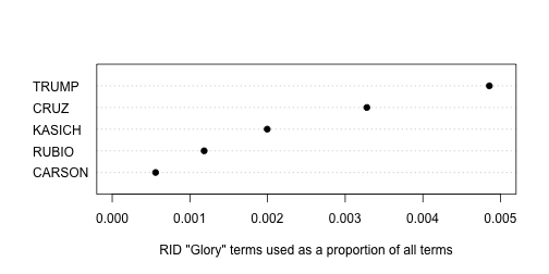
We could probably spend a whole day analyzing this information, but here, let’s simply compare candidates on their relative use of language in the “Emotions: Glory” category of the RID. We do this by slicing out the feature with this label, converting this to a vector (as there is no drop = TRUE option for dfm indexing), and then reattaching the document labels to this vector so that it will be named vector. We then send it to the dotchart() for a simple plot, showing that Trump was by far the highest user of this type of language.
canddfmRelRID[, "EMOTIONS.GLORY._"]
## Document-feature matrix of: 5 documents, 1 feature.
## 5 x 1 sparse Matrix of class "dfmSparse"
##         features
## docs     EMOTIONS.GLORY._
##   CARSON     0.0005586592
##   CRUZ       0.0032786885
##   KASICH     0.0019954390
##   RUBIO      0.0011837121
##   TRUMP      0.0048559404
glory <- as.vector(canddfmRelRID[, "EMOTIONS.GLORY._"])
names(glory) <- docnames(canddfmRelRID)
dotchart(sort(glory), xlab = "RID \"Glory\" terms used as a proportion of all terms",
         pch = 19, xlim = c(0, .005))